A plate heat exchanger has been modelled. It may not be a practical design, but it suffices for an example. It consists of 101 plates, with 100 spaces between them. Half of these are reserved for a hot water flow and the other half for a cold water flow. The two outer passes a cold and a hot one, actually have heat transfer only on one side. This could be accounted for, but this is neglected in this example.

The plate dimensions are: length 8[m], width 0.5[m] and thickness 2[mm]. The plates are Carbon Steel. The distance between the plates is 8[mm]. Thus, the total thickness of the plate package is 1002[mm]. The figure below shows the principle of the arrangement.

The process side is as follows: The hot flow is 400[kg/s] water of 80 degree Centigrade; the cold flow is also 400 [kg/s] water, but with a temperature of 20 degrees Centigrade. The arrangement is counterflow. The initial temperature difference is 60 degree Centigrade. Using a the Adams method to calculate the heat transfer coefficient and a fouling factor of 0.00005 [K.m^2/W], the total Duty is 41.16 [MW]. The thermal efficiency of the exchanger is about 41%. The traditional calculation method is here.

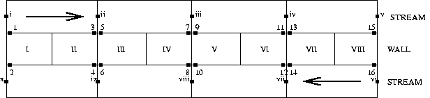
For the physical model of AHTL, the 50 passes per flow are lumped into one. The heat exchanger is divided along its length into 10 subdivisions. Although each flow has ten control volumina, the heat transfer area is divided into double that number.

This is convenient for a number of reasons. The first one is that in this way, a linear spatial distribution of the wall temperature is achieved, This gives a good approximation of the LMTD with a small number of subdivisions (Trapezium rule). Also, the extreme conditions are calculated correctly with this arrangement. Furthermore, this wall division arrangement is necessary, when a wall thickness or material change occurs or when the flow geometry changes at one of the process sides. In the figure below, the numbering scheme is illustrated. The lower case roman numbering refers to stream nodes, the capital roman numbering to the wall number and the normal numbers to the surface numbers. The figure shows four control volumes per stream, the plate exchanger example has ten control vloumes, but the numbering convention is the same.

The initial condition is a temperature of 20 degree Centigrade throughout. At t=0, the hot flow is stepped up from 20 to 80 degree C. Here is the time response of the process temperatures (Hot_in = 80 degree Centigrade or 353.15 K, Cold_in is 20 degree C or 293.15 K):

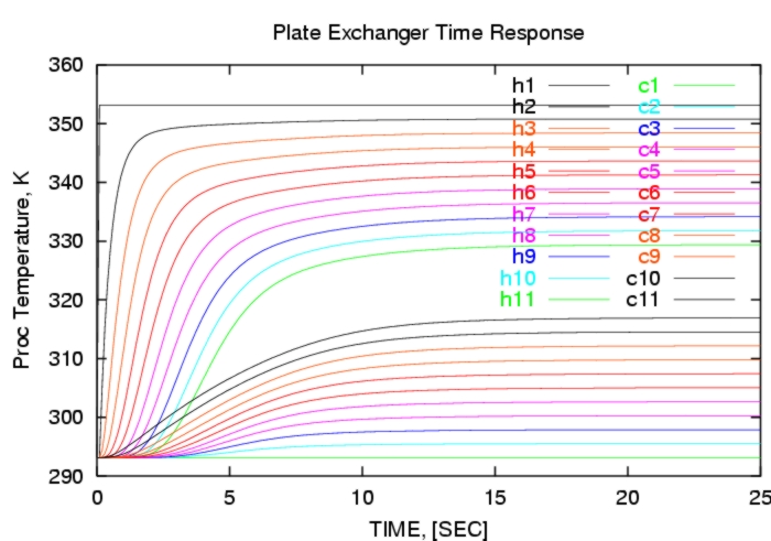
The legend: h1,h2,....,h11 indicates the hot flow nodes (one more than there are subdivisions), the legend: c1,c2,....,c11 does so for the cold flow. The index "1" indicates the inlet; the index "11" is at the outlet.

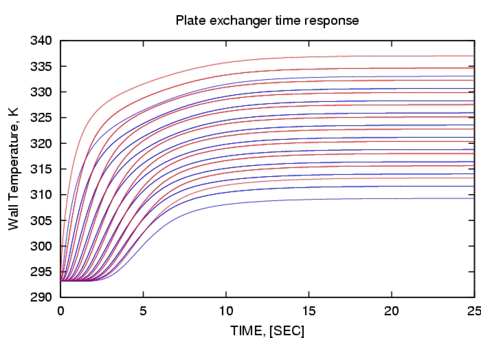
The pertaining plate wall temperatures are shown in the figure below. The red curves are the surface node temperatures at the hot fluid side, the blue curves are those at the cold fluid side. There are only eleven lines, while there are 20 wall segments. The reason for this is, that the 18 wall segment nodes at the inner nine stream nodes encounter identical operating conditions. Temperatures would differ and more lines would appear when other flow conditions or wall material/thickness/fouling would occur.

The steady-state solution can be found here. This is an unedited output of AHTL. The input files are: solid properties, wall definition file, fluid properties, stream definition file and heat transfer model definition.The output allows full cross-referencing of the fluid balances (mass-impulse-energy) whithin the fluid balance model. Further down, full output of the heat conduction model and heat transfer model is given. Last, but not least, heat flows pertaining to each of these three models can be cross-referenced between the three main models. This makes the heat transfer problem fully transparent.

AHTL offers comparable features as an equation-based model, i.e.: any quantity in the model can be accessed and inspected. AHTL has the advantage that the models provided are generic and full-engineering strength. While this would in principle be possible in equation-based form as well, it appears that, to date, this has not been done for generic heat transfer simulation.

AHTL can handle vaporizing flows and can calculate actual heat transfer coefficients based on fluid properties at bulk and film temperatures. Only the correlations are input (can be selected); all the required actual fluid bulk and film properties are collected automatically at run time. This is the power of AHTL: provide simple engineering input and get fully implemented conservation laws, rigorous engineering correlations, geometric freedom and dynamic simulation.

back